Summary

I built a renderer in C++ and OpenGL for displaying point clouds containing hundreds of millions of points in real-time. To achieve this, I implemented an octree-based Level of Detail (LOD) system from scratch. This post covers the motivation behind the project and a high-level overview of how the renderer works.

Links

GitHub

What is a point cloud?

Point clouds are 3D models made up entirely of points, rather than the polygon meshes used in traditional 3D modelling. They offer a higher degree of accuracy when representing real-world environments, which makes them a natural fit for fields like surveying and construction, where precision in the captured model is critical. Here’s a screenshot from the renderer:

Phantom Bluff Cliff Face, Lake Oswego (12.8M points).
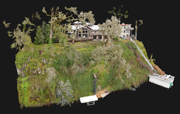
By ’TLT Photography - Aerial Mapping’ on Sketchfab

Point clouds are commonly captured using LiDAR scanners. Raw scans can contain anywhere from hundreds of millions to billions of points, depending on the scale and resolution of the capture.

The problem

Rendering point clouds with hundreds of millions of points requires an enormous amount of data to be processed in real-time (meaning a minimum of ~30 FPS). Simply rendering every point on screen is not feasible on most consumer-grade hardware, so we have to take a more sophisticated approach.

The solution

If you’ve played video games, you’ve likely come across the term LOD (Level of Detail). Games use LOD systems to optimise rendering performance by swapping in lower-detail versions of 3D assets the further they are from the camera:

Different LODs of a mesh. Image taken from this paper.

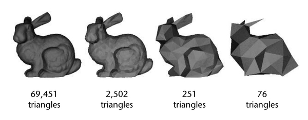
This reduces rendering workload significantly by not needlessly rendering high-detail assets the player can barely see.

My renderer applies the same principle to point clouds:

1. Multiple LODs are generated for the input point cloud
2. Higher visibility parts of the point cloud are rendered using higher-detail LODs, while less visible parts are rendered using lower-detail LODs.

Octree-based LOD system

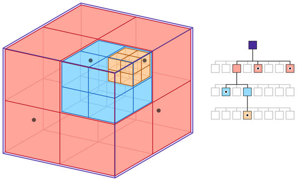
An octree is a spatial data structure that recursively partitions a cube into eight smaller cubes, known as octants. Each of those octants can then be subdivided into eight more octants, and so on. ‘Spatially aware’ just means that the data structure is based in coordinate space, so we can query the position of each octant:

Visual representation of an octree (taken from here)

So how does the software use this structure to create different LODs?

At a high level, the octree is built as follows:

1. Subdivide each node into a 3D grid using spatial hashing.
2. Insert every point in the point cloud into the root node by calling the insert() method and passing the point’s position and colour.
3. If a point falls into an empty grid cell, store it in that cell.
4. If a point falls into an occupied grid cell and the node contains fewer than minPointsPerNode points, store it in an overflow array. This prevents nodes that are mostly empty from being created, resulting in better octree traversal times due to fewer overall nodes.
5. Otherwise, recursively call insert() on the child node the point falls into. At the same time, flush all points from the overflow array into their corresponding child nodes, creating child nodes as needed. This is how the octree is recursively built.

At each level of the octree, a subsample of the point cloud is stored. Since each level is up to 8x more dense than the one above it, each level contains a progressively more detailed subsample. All nodes together reconstruct the original point cloud and no points are duplicated.

To help make that explanation clearer, here’s an image that shows how each level of the tree gets progressively more detailed:

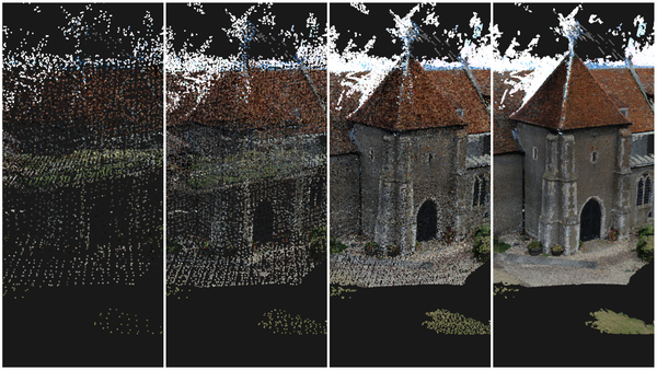
The point cloud on the very left is stored in the root node (level 0), the second is depth 1 of the octree, the third depth 2, and the fourth depth 3.

And that’s how the LOD system works. Each level of the octree represents a different level of detail, with deeper levels containing progressively more detail than those above them.

If you’d like to learn more about the implementation, I recommend reading the ‘Inserting Points’ section of this paper. The octree implementation used in this software is based on the approach described there.

The code below is my implementation of the above explanation in C++:

void OctreeNode::insert(const glm::vec3* position, const glm::u8vec3* colour) {
  // spatial hashing:
  // get the cell index of the cell this point falls into in 3D space.
  // this is the point's 3D position translated into a single integer
  int gridCellHash =
      (std::floor(position->x / cellSize)) +
      (std::floor(position->y / cellSize)) * resolution +
      (std::floor(position->z / cellSize)) * resolution * resolution;

  // if the point falls into an unoccupied grid cell, store the point there
  if (grid.find(gridCellHash) == grid.end()) {
    grid[gridCellHash] = {*position, *colour};
  } else if (grid.size() + overflowPositions.size() < minPointsPerNode) {
    // otherwise if the number of points in this node has less points than the
    // min threshold, store the point in the overflow array
    overflowPositions.push_back(*position);
    overflowColours.push_back(*colour);
  } else {
    // otherwise, call insert() on the child node that the point falls into.
    // create the child node first if it doesn't already exist.
    unsigned int childNodeIdx = getChildNodeIndex(position);
    if (!isChildActive(childNodeIdx)) {
      createChildNode(childNodeIdx);
    }
    children[childNodeIdx]->insert(position, colour);

    // the min point threshold is now surpassed, so flush all points in the overflow
    // array into child nodes (if they haven't been already)
    if (!overflowPositions.empty()) {
      for (size_t i = 0; i < overflowPositions.size(); i++) {
        unsigned int childNodeIdx = getChildNodeIndex(&overflowPositions[i]);
        if (!isChildActive(childNodeIdx)) {
          createChildNode(childNodeIdx);
        }
        children[childNodeIdx]->insert(&overflowPositions[i], &overflowColours[i]);
      }
      overflowPositions.clear();
      overflowColours.clear();
    }
  }
}

Below is the resulting octree structure from the above algorithm, visualised in the renderer:

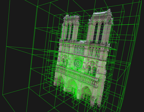
If you’d like to learn more about the formula for the value of gridCellHash (a process called spatial hashing) you can read about it in this paper, which is what I based my implementation on. This is how each node is subdivided into a 3D grid.

Rendering the point cloud using the LOD system

With the octree built, the renderer can decide which nodes to draw based on their visual importance.

There are several ways this could be done. Initially, I experimented with prioritising nodes by their distance from the camera. This worked reasonably well, but it caused too much of the point budget to be spent on nearby regions. As a result, distant regions were rendered in very low detail, breaking the cohesiveness of the overall view.

Instead, I implemented the approach described in the Potree paper, where nodes are rendered in screen-projected-size order. In other words, the nodes that appear largest on screen are rendered first, followed by progressively smaller ones. This produces a more cohesive view of the point cloud, without abrupt transitions in detail.

The implementation works as follows:

1. A user-defined points-per-frame budget is set. This can be increased for higher detail or reduced to improve performance on less capable hardware.
2. All nodes are collected into an array and sorted by their projected size on screen.
3. Nodes are drawn in sorted order until the point budget is exhausted.

Rendering the octree with OpenGL

A significant part of this project was learning OpenGL and linear algebra in the context of graphics programming in order to implement the 3D renderer from scratch in C++. I won’t go into how the 3D rendering pipeline itself is implemented as there are plenty of excellent resources online that cover it far better than I could here, and it’s not unique to this project.

What I will briefly cover is how the rendering data is organised and sent to the GPU, as that part is specific to this project. Some familiarity with OpenGL will help here. Each node is associated with three buffers:

• A vertex buffer for position data
• A vertex buffer for colour data
• An index buffer for the node’s bounding box geometry

Each node also has a VAO that stores its vertex attribute configuration. When it comes time to draw, the current node’s VAO is bound and glDrawArrays() is called, rendering the node’s points to the screen.

There is certainly room to optimise this further, but for the scope of this project it performs well enough, and refining the OpenGL implementation is something I’d look to revisit with more experience.

Measuring performance with SDL

To measure performance, I time each frame by starting a counter at the beginning of the rendering loop and stopping it at the end.

This is done using two SDL functions: SDL_GetPerformanceCounter(), which returns the current value of the system’s high-resolution counter (you can think of this value as the number of ticks that have elapsed since the system started) and SDL_GetPerformanceFrequency(), which returns the number of ticks in one second.

Dividing the elapsed ticks by the frequency gives the frame duration in seconds, from which both milliseconds and FPS can be derived:

void Timer::start() {
  startTime = SDL_GetPerformanceCounter();
}

void Timer::end() {
  endTime = SDL_GetPerformanceCounter();
  elapsedMS =
      static_cast<float>(endTime - startTime) /
      static_cast<float>(SDL_GetPerformanceFrequency()) * 1000.f;
  FPS = static_cast<int>(1000.f / elapsedMS);
}

glFinish() is also called before stopping the timer each frame. This forces the CPU to wait until all queued OpenGL commands have finished executing on the GPU. Without it, the measured frame time may not include all of the rendering work, resulting in performance figures that are artificially low.

Results

I tested the renderer on two systems: an M1 MacBook Pro and a PC equipped with an i9-10900K and RTX 3080.

For a point cloud containing 330 million points, the LOD system improved performance on the PC from approximately 3 FPS to 60 FPS.

On the MacBook Pro, rendering all 330 million points without the LOD system caused the machine to become unresponsive. With the LOD system enabled, the renderer achieved approximately 40 FPS.

All tests were performed using a points-per-frame budget of 20 million points.

Despite rendering only a fraction of the original dataset each frame, there was no noticeable loss in visual fidelity when compared to rendering all 330 million points. The LOD system therefore provides a substantial performance improvement while preserving a faithful representation of the original point cloud.

The images below show this comparison. The first image was rendered using the LOD system with a points-per-frame budget of 20 million points. The second image shows the same point cloud rendered in full, with all 330 million points visible:

‘Elmstead’ rendered using the LOD system with a 20M points-per-frame budget.

‘Elmstead’ rendered with all 330M points, without the LOD system.

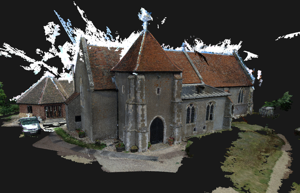
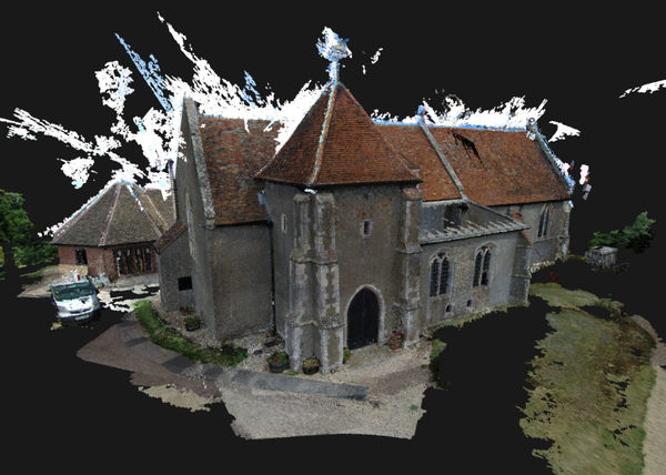
As shown, the visual difference is almost indistinguishable, despite the first image rendering at approximately 60 FPS and the second at approximately 3 FPS.

Using the software

Instructions for building and running the software can be found in the GitHub repository.

The user interface is currently quite minimal, as I didn’t have time to implement a GUI during the project. Most configuration is therefore done through command-line arguments.

Conclusion

I learned a lot from building this project. It was especially fascinating to see how an abstract data structure like an octree can be applied to solve a real-world problem.

I’ve intentionally kept the explanations in this post fairly high-level, as my goal was simply to convey the core ideas behind the LOD system. Topics such as shaders, camera controls, and user input handling were omitted because they are relatively standard and not central to the renderer itself. If you’re interested in the complete implementation, feel free to explore the codebase.

There is also plenty of room for further improvement. One obvious optimisation would be view frustum culling, which would prevent nodes outside the camera’s view from being considered for rendering. The codebase itself could also benefit from a cleanup, as it’s far from the prettiest C++.

Overall though, the project achieved its primary goal: making extremely large point clouds practical to explore interactively.